Explainable AI

There is a frequently used argument that favors using simpler model: “we need an easy model to explain to our business partners.” Modelers usually buy into this argument and develop models that do not capture all the valuable relationships present in the data.

Business problems are usually complex. Expecting that linear models will handle non-linearities, data quality issues and high dimensionality is unrealistic. Should we sacrifice performance for explainability? The answer depends on the specific business problem, but I would expect that most of the time performance (that is translated in business value) is more important. There are multiple tools in data science that help us to interpret models that are considered black boxes.

There are three types of model interpretability that are useful and applicable to almost all models:

• Global interpretability: This helps us to understand how the model predictions are related to the input variables. This interpretation is concerned with a general understanding of the model’s inner works and drills into an individual case example.
• Cluster explainability: This is used to explain how the model works when we control by sub- populations (cohorts).
• Local interpretability: This gives insight into how specific factors influence a single model prediction compared to a baseline prediction. This is meant to explain how observed variables influenced the prediction in a positive or negative way for a particular subject or observation.

There are three main methodologies to achieve interpretability:

• SHAP (SHapley Additive exPlanations) is based on game theory and these values reflect the optimal way of attributing credit of a prediction.
• LIME analyzes the individual prediction and generates imaginary observations and sees whether the model changes the prediction.
• Anchor tries to generate a set of rules that will encapsulate a prediction.

I will use a problem to illustrate how to use these tools. Mortality is a problem that is clearly non- linear and very complex with many iterations between explanatory variables. You can follow the code used at https://github.com/cbrioso/Miscellaneous/blob/main/Mortality%20Shap.py

I use data from an Epidemiologic Follow-up Study from the CDC (https://wwwn.cdc.gov/nchs/nhanes/nhefs/) and fit a mortality machine learning model (Xgboost). The set of predictors are intuitive: age, gender, BMI, etc. For model explanation I use SHAP values. I won’t get into details regarding how these values are derived, but will put emphasis in their interpretation. However, documentation for SHAP and LIME are readily available.

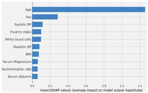
First, we want to understand what variables are the more impactful for explaining mortality. This is clearly observed in the Feature Importance plot. As expected, age and gender are the more important variables in the model. Other important variables are Systolic BP, Poverty Index, and BMI (body-mass Index). These variables make sense and concur with our understanding of mortality. (See Figure 1)

Figure 1 Feature Importance Plot (Top 10

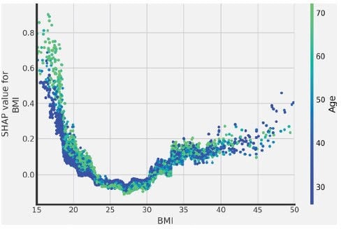
Once we understand the major drivers of mortality, we are interested in the relationship implied by the model. This can help us to bring intuition to relationships that we don’t know or (sometimes more important) to confirm the reasonability of the relationships that we know. Let’s take as an example BMI: very high and very low BMI values are related with higher mortality. This is aligned with expectations. Moreover, we observe that this relationship is different for younger and older populations. Mortality for people with low BMI is even higher for older people. (See Figure 2)

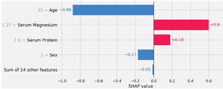
Finally, we are interested in understanding model predictions for a specific individual relative to an average subject. In Figure 3 we observe factors that influenced the predicted mortality for the first individual in our sample. Two factors: age and gender move the prediction to be a relative lower than an average subject. However, Serum Magnesium and Serum Protein are factors that have an adverse effect in the forecast mortality for this subject.

Figure 2 Relationship Between Mortality and BMI

Figure 3 Individual Risk Explanation

As demonstrated in this example, a machine learning model can easily be interpreted. Tools like SHAP, LIME and Anchor can facilitate the understanding of the model and the business problem. Let’s make full use of the tools that we have in hand to build better models and communicate how predictions are generated.