Analyzing and Predicting Policyholder Behavior at Policy-Level with Machine Learning: Part 1 Traditional Experience Studies and Assumption Setting Methods
By Shaio-Tien Pan
The Financial Reporter, September 2024

Traditional insurance business involves pooling risk from individual policyholders, and while it is impossible to accurately predict what will happen to every life, insurance companies rely on robust estimates of various rates (e.g., mortality rates, lapse rates) and the law of large numbers for an accurate prediction of aggregate claims. Actuaries are trained to determine and analyze these rates and probabilities based on experience data, and then use them to develop assumptions for pricing and valuation. The process typically involves grouping the experience data into cells and computing the experience rate for each cell by dividing the total event by the total exposure.
Although the experience study methodology described above is standard and has been practiced by actuaries for decades, there is one notable limitation with the methodology: A given policy’s experience over time is being treated as if they are independent exposures. While the independence assumption may be reasonable for mortality, it is questionable for many other behaviors. For example, industry experience has shown strong serial correlation in policy-level withdrawal amounts over time. On a couple of large variable annuity with guaranteed lifetime withdrawal benefits (VA GLWB) blocks we find that almost 90% of policies that took the maximum allowed withdrawal amount (MAWA) in one year would do the same the next year, while about 80% of policies that withdrew for less than the annual maximum amount would remain under-utilized (and often withdrawing the same dollar amount) in the subsequent year. In addition, a significant portion of policyholders with tax-qualified funds took exactly the required minimum distribution (RMD) amount year after year, regardless of the GLWB benefit. These data suggest that instead of being independent from one year to the next, most policyholders are remarkably consistent in their behavior over time.
Given the stickiness in individual behavior, it would seem reasonable to make assumptions about each policyholder’s future behavior using that policy’s distinct transactional data, yet that’s rarely done in practice. Making accurate policy-level assumptions has never been a goal for actuaries, who are trained to think in terms of aggregate-level metrics such as average. If there are two identical GLWB policies and one is withdrawing 100% of MAWA while the other is taking 90%, many actuaries would be tempted to assume and model both policies as if they are each taking the average withdrawal rate of 95%. The actuaries may even claim victory for achieving “100% overall A/E” for the 95% withdrawal rate assumption. However, due to non-linearities in the liability, using the average assumption may significantly underestimate the aggregate reserve. This can be proved using Jensen’s Inequality (see Appendix), but we will illustrate the idea using the simple GLWB example above: Let’s say account value will run out if the withdrawal amount each period is greater than 96% of the MAWA; if we assume both policies to take 95% of MAWA, the total projected claims would be 0, which is clearly nonsensical since the account value will be depleted for the policy withdrawing 100% of MAWA. Therefore, setting assumptions more accurately for each policy (e.g., 100% for the first policy and 90% for the second) is not just a nice-to-have, but is necessary for accurate aggregate claims estimate.
In summary, traditional methods for experience studies and assumption settings contain several fallacies. By grouping experience data together based on some attributes, they fail to properly capture and utilize each policy’s idiosyncratic, yet persistent, behavioral patterns. Traditional methods also tend to set assumptions at too high a level, resulting in underestimation of reserves when the liability is non-linear with respect to the underlying assumptions.
This series of articles[1] proposes a novel, machine learning approach to analyze the experience data and predict future policyholder behaviors. The model takes as inputs a policy’s transaction history as well as other demographic and policy attributes, and outputs a realistic sequence of future actions that the particular policy is likely to make over time. In the following sections we describe the model’s input and architecture in detail, using a block of VA with GLWB as an example for illustration purposes. The model enables actuaries to efficiently analyze and set assumptions at policy-level granularity, which improves reserve estimate. The model is also capable of predicting multiple behavioral events while capturing the interrelationships between them. In addition, an artifact of the model is a learned representation of a policy’s behavioral pattern, which can be used for policyholder segmentation and other purposes.
Model Description
Data
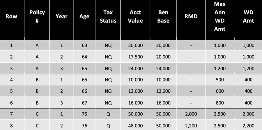
Typical experience studies data looks like Table 1, where each row of the dataset represents a combination of policy and time (policy year in the example, but could also be monthly and calendar year-basis), and contains information about the policyholder, product, and the outcome of the event of interest (withdrawal amount in the example).
Table 1
Experience Studies Data are Usually Organized into Rows of Exposures: Policy and Year in this Example
Traditional experience studies implicitly assume that the exposures (i.e., the rows in the table) are independent, and actuaries would typically aggregate results such as average withdrawal percentage by some attributes in the dataset that the actuary has identified to be drivers of the outcome. For example, Row 3 and Row 4 in the table might be grouped together if the actuary decides tax status and age are influential to GLWB withdrawal behavior.
In contrast, our approach slices the experience data by policy, preserving the valuable information contained in the sequence of transactions each policy has made. For example, it appears that Policy A always maximizes the GLWB benefit, Policy B seems to withdraw the same dollar amount every year, while Policy C withdraws based on the RMD requirement. The unit of account under our approach is a policy, and we view the data in Table 1 as three data points.
Generally speaking, our approach categorizes each policy’s data into the following:
- Static data Xstatic: Includes demographic information such as gender, tax status, and policy or product information. Static data generally remain unchanged during the lifetime of a policy.
- Current snapshot data Xt: Refers to current values of time-varying variables, such as account value, guaranteed amount, policy year.
- Historical transactions up to time t-1 H= {τ1 , τ 2,…, τ t-1}: A timeline or a sequence of a policyholder’s past decisions, and the context under which these decisions took place.
Specifically, each transaction τ k is defined as a tuple (i.e., a vector of values) of (Ck, Yk): - Contextual information Ck. Policyholder behavior is dynamic and often influenced by the capital market condition, account performance, and other observable factors that may be in the experience data. Juxtaposing the context and decision together helps the model infer a policyholder’s hidden attributes, such as levels of risk tolerance, market sensitivity, or cash needs, all of which are useful for predicting future behaviors.
- Policyholder decision Yk, such as surrender, or taking a $W withdrawal, etc. Note that taking no action during a period is one of the possible decisions. A policyholder’s inactivity is informative.
- The policy’s decision at time t Yt
Note that because we are slicing the experience data more granularly (policy-level rather than grouping the data into a few cells), our model needs to be able to digest and analyze a much higher volume of data, and that is where machine learning[2] excels.
Modeling Considerations
While our goal of using machine learning to discover patterns in experience data and utilizing them to predict future policyholder behaviors seems like a typical data science problem, there are several unique challenges in this use case. First, the experience data consists of a mixture of time-series and tabular data. Most off-the-shelf machine learning models require the input data to be either exclusively time-series or tabular. Second, the target variable, in this case future policyholder behavior, is not straight forward to define because the policyholder may possibly have an infinite number of choices, and it is not even clear if the model should be formulated as a classification or a regression problem. The decision to lapse or not seems like a classification problem, while the withdrawal amount is a continuous variable and more akin to a regression problem. Lastly, insurance products are long term and insurers and actuaries are interested in predicting not just what the policyholder will do next period, but in each period over the next 30 or 40 years!
These challenges call for a custom model. Part 2 of this series will explain our model architecture and how it addresses each of these issues.
Appendix
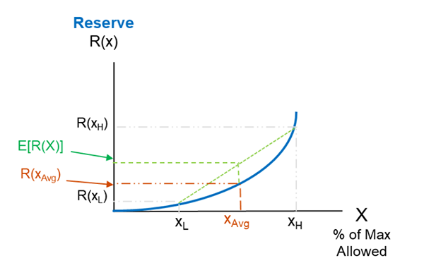
Due to optionality and other reasons, many actuarial reserves are non-linear and convex with respect to underlying variables and drivers. For example, if we plot the GMxB reserve (PV of claims) versus annual withdrawal amount for VA GLWB, we’d expect it to look like the blue curve in Figure 1 below.
Figure 1
Graphical Illustration of How Using the Average Assumption would Underestimate the Reserve when the Reserve is Convex with Respect to the Assumption
As the annual withdrawal amount goes up, the reserve is expected to rise rapidly because not only does the probability of claim occurrence (i.e., account value depletion) go up, but claims will happen earlier so they will be paid out for more years and with less discounting.
Letting X be the annual withdrawal amount, since the reserve function R(X) is convex, using Jensen’s Inequality:
In other words, if say half of the block withdraw XH while the other half withdraw XL, and if XAvg is the average of XH and XL, then we can show that the total reserve calculated using the average assumption will be less than the total reserve calculated using a more granular assumption:
Statements of fact and opinions expressed herein are those of the individual authors and are not necessarily those of the Society of Actuaries, the newsletter editors, or the respective authors’ employers.
Shaio-Tien Pan, FSA, MAAA, is a director at PwC. He can be reached at shaio-tien.pan@pwc.com.
Endnotes
[1] This article is the first of a two-part series. Part 1 discusses the limitations of traditional experience study methods that actuaries have been using for decades and introduces an alternative approach—a novel machine learning model, to analyze and predict policyholder behaviors. Part 2 (to be published in a future issue of The Financial Reporter) will describe the model’s architecture, performance and applications in detail.
[2] In recent years a growing number of insurers have started using machine learning techniques in experience studies and assumptions setting. However, in cases we have seen, their machine learning models consider one data point to be a row (i.e., an exposure unit) in the dataset like Table 1, and therefore similar to traditional methods, they fail to capture the strong serial correlations in policy-level transactions. We believe our proposed approach of setting the unit of account at the individual policy level is unique in the industry.


