Challenges of Managing Interest Rate Risk: Part 4—How to get the Most Insight out of a Company's Assets and Liabilities
By Dariush Akhtari
Risk Management, September 2024

This part will highlight the issue that the sum of key-rate metrics does not add to metrics derived by parallel shift to the entire curve, even at very low shift size and how to define a single rate change to be applied to a key rate (or the entire curve) since the rate changes are generally not level or parallel.
In the next part, I will evaluate various methods used to combat the non-additivity of the key rates.
Non-additivity of Key Rates
Previously I indicated that for interest-rate sensitive instruments the use of smaller shift sizes produces KRkDV01s with a sum much closer to DV01, whereas larger shifts would not. This is due to two main reasons. First, with larger shift sizes, the higher rate changes may trigger cash flow changes causing larger interaction between the key rates. The second, is that with larger shifts, there is a higher chance that one of the shifted rates would cross a point of inflection.
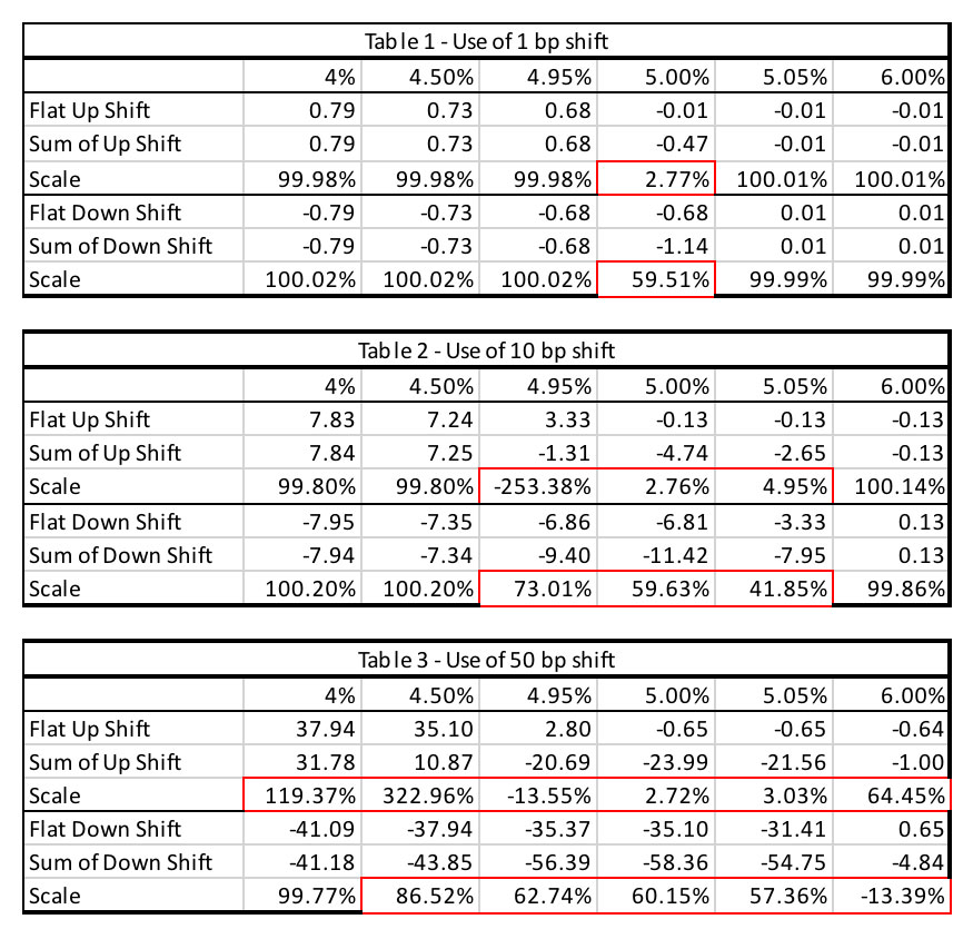
To explore how close the sum of KRkDV01s is to DV01, we could use a scale to reflect the ratio of DV01 to the sum of KRkDV01s, or more appropriately, their subcomponents, i.e., values using up and down shifts. Obviously, the closer the scale is to 100%, the closer the sum of KRkDV01s is to DV01. One could get far closer to 100% when the shift size is 1 bp but could be very low (say 2%) or very high (say 400%) when a 50-bp shift is used. In fact, the closer to the inflection point one gets, the farther away the scale would be from 100%. Tables 1, 2 and 3 in Figure 1 highlight how various shift sizes impact this ratio (i.e., the ratio of change in value due to a flat up/down shift to the entire curve versus the sum of the changes in value when the same shift size is applied to parts of the curve to capture the key rates). The issue is exacerbated the closer one gets to the inflection point and when the shift size is larger.
Figure 1
Tables 1 – 3: Impact of Difference Curve Shift Size on Scale
From the tables in Figure 1, it can be noticed that both larger shift sizes and proximity to the inflection point result in the scale to be materially away from 100%. The approach provided in Part 2 of this article series can also be applied to key rates to identify to what level of rate change one could rely on the approximation validity of the key rates. Additionally, use of cumulative key rate calculation incorporates cross key rates and would improve the approximations using key rates.
How to Calculate Rate Change to Apply to Metrics
To use ALM metrics, one needs to know by how much rates have moved. I compared three different approaches.
Average of Rate Changes
This approach simply takes the average of all rate changes over the period used. For example, for key rate 5 the average of rate change in years two to 10 would be used and in a parallel case the average of rate change on the entire curve would be used. This approach suggests that all periods have an equal weight.
Calculated Yield Change
One could convert the entire spot curve to a yield by calculating an internal rate of return (IRR) of the cash flows to their discounted value. Similarly, after a rate change, calculate a yield by taking IRR of the same cash flows to their discounted value using the new rates. The change in this yield versus the original is the change to be used for that key rate. Note that one could always consider the entire curve as one big key rate.
Weighted Rate Change (the Proposed Approach)
To account for the unequal weight a cash flow has on the discounted value, I propose weighting the rate change for each period based on the ratio of the discounted value of that period’s cash flow to the total value as explained in Appendix 1.
Comparison of Rate Change Methods
I compared the absolute error of the approximated value using a 1-bp shift for the change to the entire curve (i.e., using DV01 and CV01) for the A cases (will be defined in Part 5) as seen in Table 4. As it can be observed from Table 4, the weighted cash flow approach seems to outperform the other approaches in calculating a single rate change to be used for the key rate.
Table 4
Comparison of Various Rate Change Methods on Entire Curve
Appendix 1
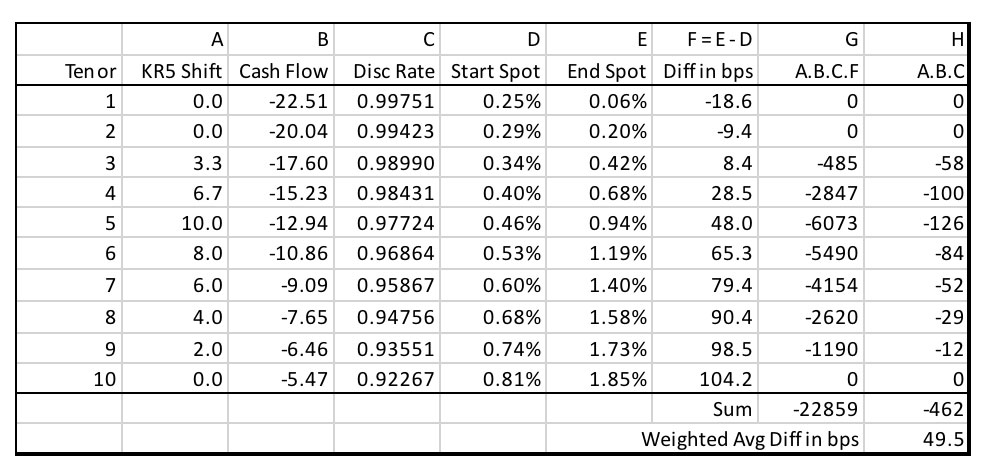
Below is the recommended weight used to compress the change in rates within the periods in a key rate to a single rate to be used with KRkDV01 and KRkCV01. Note that this method is also suggested to be applied to the entire spot curve change for use with DV01 and CV01. To calculate a weighted shift, consider Table A1.1.
Column A represents the shift applied for the particular key rate (KR 5 in the below example using 10 bp shift). Column B is the calculated cash flows using the beginning of period spot rates (i.e., column D). Column C represents the discount rate (discount rate (t-1) / (1+spot rate (t) in D) that when applied to the cash flows and summed would produce the value of the instrument. Column E is the spot rates for the period the value of the instrument is to be approximated. Column F is simply the difference of columns E and D. Column G is the product of columns A, B, C and F. Column H is the product of columns A, B and C. Finally, the weighted average of the rates used with the particular key rate is the ratio of sums of columns G and H.
Looking at column F, it would have been hard to choose a single rate to be used with KR5DV01/KR5CV01. This method suggests that for this set of cash flows 49.5 bps should be applied to key rate 5.
Table A1.1
How to Calculate Weighted Rate Change
Statements of fact and opinions expressed herein are those of the individual authors and are not necessarily those of the Society of Actuaries, the newsletter editors, or the respective authors’ employers.
Dariush Akhtari, FSA, FCIA, MAAA, is chief actuary at Converge RE. He can be contacted at dakhtari@converge-re.com.


