Strategic Risk Management: How to Engage the C-Suite

By Damon Levine

Risk Management, September 2024

Strategic Risk Management (SRM) is typically described as a program, or set of processes, for identifying, quantifying and mitigating risks that affect a company’s strategic objectives and their execution. This may be a stand-alone framework or a part of an Enterprise Risk Management (ERM) program. However, there are specific techniques SRM may employ to capitalize on its primary focus of strategic execution. 

To ensure engagement from the C-Suite and Board members, we focus on SRM tools and techniques that:

• Articulate challenges to strategic execution,
• prioritize risks to attaining objectives,
• drive key performance metrics, and
• improve the chance of success.

To make these ideas more concrete we use a global insurance company as an example.

The Strategy Survey

A key step is to articulate strategic objectives and determine the primary challenges to their execution. A 30-minute survey sent to management, department leaders, and other key decision-makers will get this done with minimal pain.

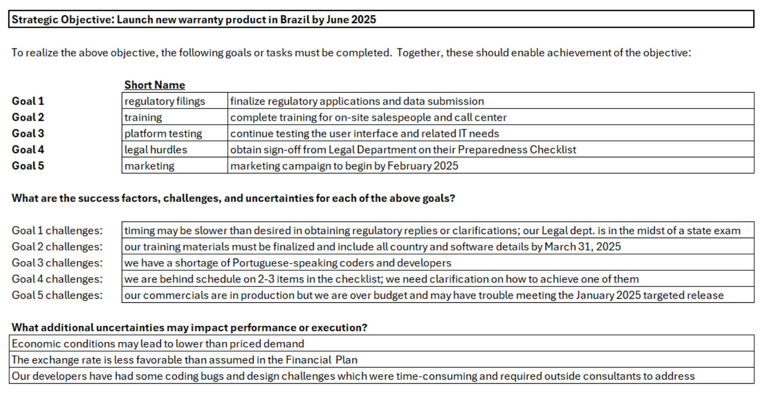
We ask each survey participant to list two to three strategic objectives on which they are focused over the next 12 months. For each strategic objective, the respondent considers key foundational projects or prerequisites. These are tasks or goals that, once realized, should enable achievement of the overall strategic objective. In Exhibit I, they are referred to simply as “Goals” and the simple message is that if we succeed on Goals one through five, we are confident we then achieve the strategic objective.

Exhibit I
Sample Survey Replies for a Strategic Objective

In the above, the respondent lists a strategic objective for a new warranty product launch in Brazil.

After describing the objective, several foundational tasks, labeled Goal 1 to Goal 5, are listed. Finally, the challenges or uncertainties related to each goal are listed.

Note that we have not used the word “risk” at all, but we have carried out practical and detailed analysis of execution risks for this objective. It is best to avoid the word risk in many circumstances because there are differing opinions about what risk is. We then may easily obtain some additional detail through a brief discussion with those knowledgeable of the current risk mitigation or controls. We then have a useful summary of risk and risk response information in Exhibit II.

Exhibit II
Illustrative Strategic Risks and Response

Expert Input for Risk Assessment

We have identified key strategic risks, existing mitigation, and potential action needed to improve our management of these risks. Due to time and resource constraints, it is likely impossible to address all of these simultaneously. For this reason, we need to prioritize risks in order to guide management’s decision on financial and resource investments in improving risk responses. 

We have identified the following challenge we refer to as Risk X: “We have a shortage of Portuguese-speaking coders and developers.”  We meet with several subject matter experts (SMEs) among our colleagues in strategy, IT, and software development, as they are most familiar with this challenge.

We communicate the metric with which we want to quantify the risk, e.g., GAAP earnings impact on our product launch, versus our baseline forecast for earnings from this initiative. 

We ask the SMEs a simple question: Assuming the risk has manifested, what are your best guesses for:

• The minimum impact: a;
• the mode, which is simply a “best guess” or expected impact: b; and
• the maximum impact: c.

Impact should consider, for example, effects of a delay from coding, excess need for debugging or testing, or other poor performance on this software development challenge.    We have the following reply from one SME:

Exhibit III
One SME’s Impact Estimates for Risk X

We have three numerical estimates as above from each SME. A simple way to make use of all of this is to compute the average for each of the above three values. So, we now have the following based on the average of all of the SME responses:

Exhibit IV
Averages of All SMEs’ Impact Estimates for Risk X

This data serves as a basis for risk modeling of Risk X. As we have minimum, mode, and maximum parameters we can use a statistical distribution called the Expert’s Distribution or PERT.  “PERT” stands for program evaluation and review technique, the first well-known application of this distribution in the field of project management. 

The Expert’s Distribution is an intuitive moniker for this distribution as we should feel comfortable asking the expert for these three estimates that are its parameters. If instead we ask directly for a statistical distribution, we often receive a blank stare, or worse yet, a laugh.

The key messages of Exhibit IV are that if Risk X occurs, then (1) the impact is very likely to be between 29 and 513, and (2) our best estimate for the impact of Risk X, only knowing it has manifested, is 147.   

We can think of (1) as saying “we are 90% confident the actual impact would lie between 29 and 513” but the value of “90” is arbitrary and we are simply expecting the experts to give us a range wide enough to cover “most” situations. The mode estimate suggests that the “147 neighborhood”, e.g., 147 +/- 5 = (142, 152), is the most likely outcome across alternative neighborhoods.

Risk Quantification that Captures Uncertainty

We never know what risks will manifest nor the effects of those events. By definition the effect of a risk is unpredictable. We make use of the Expert’s Distribution to naturally express this uncertainty, which is the essence of risk. A wider distance between the minimum and maximum parameters communicates more uncertainty, less understanding of the nature of the risk, or both. We construct a simple risk distribution that illuminates our view of how the risk may “play out.” We will have a view of potential impact outcomes and understand we are more confident in actual impacts being closer to the mode.

The risk quantification approach is simple enough to carry out in the standard Excel platform, or, if desired, made easier by using any one of several add-ins available on the market. The following notions are important for the risk modeler/model owner to understand:

The parameters a, b and c (the minimum, mode and maximum) completely characterize the distribution, and we may specify the distribution as PERT(a,b,c) without ambiguity. The distribution’s mean and standard deviation are functions of these three parameters:

Note that the first equation tells us the mean (or expected value) of the distribution is a weighted average with weights for a, b and c being 1, 4 and 1 respectively. Also, the probability density function (like the “bell-shaped curve” for a normal distribution) is highest at b, and zero at the endpoints of a and b. Exhibit V shows graphs of the densities of a few different PERT distributions. 

Also, the volatility or uncertainty, as measured by standard deviation, is proportional to the width of our “confidence interval” of (a,c).

Exhibit V
Probability Density Functions for Various PERT Distribution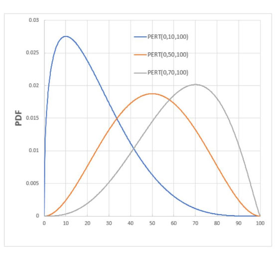

Source: https://commons.wikimedia.org/wiki/File:PERT_pdf_examples.jpg

Based on the analysis described above, we can compare different strategic risks that affect our ability to execute the product launch in Brazil. We now look at some ways to compare and prioritize the various risks identified.

Risk Prioritization

We may use a risk prioritization approach based on examining the mean and standard deviation of each risk’s impact to the strategic objective. Note that the (positive) parameters in Table 1 below represent a reduction in earnings or cashflow (whatever the choice of metric was) related to the objective’s baseline forecast.

Table 1
Summary of PERT Distributions Employed

We summarize the risks using mean and standard deviation in Exhibit VI.  We use the mean +/- 1 standard deviation to highlight a “fairly likely” range of potential results.

Exhibit VI
Illustrative Loss from Risks to Strategic Goals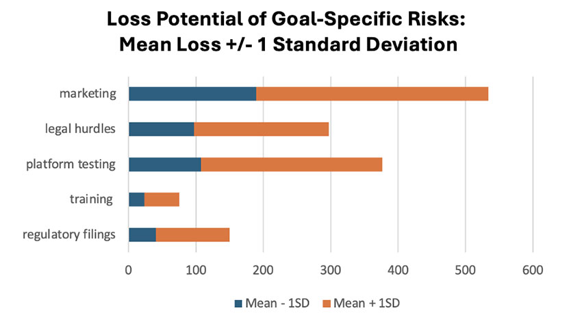

Generally, there is no method to objectively rank risks in business. Holistic comparisons require assessing one statistical distribution versus another. In the situation above, we might expect that management views “marketing” and its associated identified risk of commercial production timing and budget challenges as “rank 1,” or the highest priority.  This means that further action, time, or resources should be prioritized to further mitigate this risk. Cost-benefit analysis should also be considered as additional expense is always a reality for tactical changes or mitigation improvements.

Management may view the training issues as less of a priority and eschew any additional resources for this aspect, a “make do with what you have” viewpoint.

A Risk-Based Financial Plan

In our product launch example, we do not consider any “upside” or possible benefit from the indicated risks. This is due in part to the nature of the risks we have examined. For example, there is no meaningful upside to the “legal hurdles”; it doesn’t make sense to think of the product launch going better than expected because the product was made “very” legal. A similar view can be taken for testing, training and regulatory filings.  Perhaps we can have an exceptional marketing experience, but practically speaking, analyzing the possibility of better-than-expected impact from marketing will not influence action or help us achieve the objective. It would be an academic exercise.

All of this belies a critical element to risk management: Risk or uncertainty analysis should generally consider both upside and downside. This can be accomplished by using a PERT distribution for a risk where a<0 and c>0, which means the distribution allows both negative and positive impact to our performance metric. 

An important application of risk analysis capturing upside and downside is a risk-based financial plan. If we choose to use statistical distributions for each risk affecting results, we will likely have a fairly large number of risks. In this situation one should consider correlations across the risks. If one models each risk on its own, with PERT distributions for example, there are methods to combine them with a target correlation matrix. An approach to capture correlations across various risks which keeps these “marginal” distributions intact was previously described by the author in detail.[1] However, here we illustrate a simpler approach, without requiring correlations.

The typical financial plan of an organization is a best-estimate or baseline forecast for earnings. It is almost impossible in practical terms to gauge how hard it is to achieve the plan or how likely we are to miss it. If the CEO is tasked with defining executive bonuses based on achievement versus the plan, this presents a significant challenge.

If we determine the primary drives of earnings and sources of variation and estimate how they help or hurt our pursuit of the plan earnings forecast, we can create a risk-based plan that is above and beyond the traditional point-estimate or “one number” best guess used at most companies. It will include that best guess but will also show a possible range of outcomes resulting from how the various uncertainties play out, and it will offer a view of the likelihood of earnings outcome ranges.

The financial plan’s forecast of earnings is assumed to be wrong. We are aware of many business drivers or uncertainties (collectively, “BDUs”) that will influence our actual earnings results. These include factors we may influence and also those we cannot. They include project management effectiveness, risk response, execution on tasks, compliance, supply and demand, interest rates, accounting treatments obtained, customer behavior, taxes, pricing decisions, inflation, FX rates, employee turnover, macroeconomic forces, accuracy in data usage, company models, competition, etc. We determine a short list of those deemed most critical: BDU 1, BDU 2, etc. Many of these have upside and downside potential and it is important we capture both, without a bias. 

An attempt should be made to define each BDU so it has low or no correlation with other BDUs. For an insurer, larger than expected flood claims have a low correlation with the return on invested assets, and for a bank, higher than expected credit losses in a loan portfolio are generally not correlated with unexpected expenses for customer credit monitoring after a data breach.

Through risk interviews, surveys, or as part of the financial plan process, we have identified these uncertain factors driving earnings results and obtained SME views on their possible impacts. If the financial plan assumes an outcome or range for one of the BDUs explicitly, and its actual behavior “goes according to plan,” we interpret this as a zero impact on earnings. So, we are interested in how the uncertainties add or subtract from the plan forecast. We must first define for each BDU the probability of landing in each range of reduction or increase to plan earnings. The following shows these estimates based on SME input and available data.

Exhibit VII
Probability of Dollar Effects on Earnings by Business Driver/Uncertainty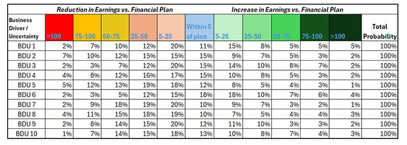

We will be simulating the possible effects of each BDU separately. Consider BDU 1. We can generate a random number from (0,1) in Excel as “rand()” and then use a simple rule to map it to the appropriate entry in its row: The simulated impact to earnings. This rule for mapping is based on forming ranges whose widths correspond to the probability estimates in the BDU’s row. Given a random value, p, from (0,1), we define the simulated effect as follows:

• For p<0.02, the impact is in the left most (red) cell, a reduction in earnings “>100”
• For p in [0.02, 0.02 + 0.07), or [0.02,0.09) it is a reduction of “75-100”
• For p in [0.09, 0.09 + 0.10), or [0.09,0.19) it is a reduction of “50-75”
• For p in [0.19, 0.31), it is a reduction of “25-50”
• …
• …
• For p in [0.95,1), it is an increase of “>100”

The same approach allows rules for any random number to be mapped to the simulated impact for that specific BDU. As a result, using 10 random numbers from (0,1) we have 10 simulated impacts to the financial plan earnings forecast. That counts as a single simulation of all of the risks’ combined effects to earnings and is illustrated here:

Exhibit VIII
A Simulation of BDU Impacts for One Simulated Year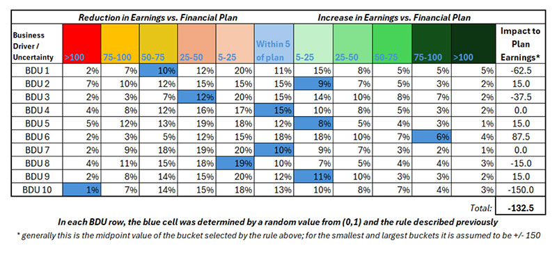

The above is one simulation based on 10 randomly simulated values in (0,1). We add the total impact of -132.5 to our plan forecast of, e.g., 1000, to obtain a simulated outcome of 867.5. If we perform this many times, we can then examine the resulting simulations to find percentiles for earnings results. Some adjustments can be made to assign more probability to tail results in order to remedy our lack or correlation, but generally the tails are not something we can model well with this procedure. However, our careful selection of the BDU categories will have ensured most correlations are low, and extreme results are not what we are attempting to model.

This allows us to state an estimated probability of actual earnings being in a certain sub-range or the probability of earnings being above or below a fixed threshold of interest, such as 110% of plan or less than 80% of plan. Such analysis holds tremendous interest to business leaders, the C-suite, the board, and also helps in implementing economic capital or risk buffer notions. It is also a valuable tool for a CEO who wishes to define bonus payouts, a priori, based on actual earnings results versus plan.

Conclusion

With a focus on the four desired attributes of SRM techniques, we are able to analyze uncertainty in strategic execution. Because we begin with the right end in mind, those four attributes with the mnemonic of PAID, allow us to build buy-in by design and communicate risk intelligence that resonates with leadership. Naysayers may always point to our inability to make predictions; this is not the point. The old saying from George Box is true: “All models are wrong, some are useful.”

Statements of fact and opinions expressed herein are those of the individual authors and are not necessarily those of the Society of Actuaries, the newsletter editors, or the respective authors’ employers.

---

Damon Levine is an enterprise risk management practitioner and consultant. He can be reached at damonlevineCFA@gmail.com.

Endnote

[1] https://www.soa.org/globalassets/assets/files/resources/essays-monographs/2016-erm-symposium/mono-2016-erm-levine.pdf